


April 23, 2007
Case Notes 9
Your basic Bayes' Theorem is an uncontroversial result in probability theory relating the conditional probabilities of two events. It is expressed like this: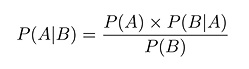 P(...) here means "the probability of ..." and the vertical bar | stands for "given". The P(A|B) bit on the left is called the posterior probability; the P(A) on the right is called the prior. The world of "before" is divided from the world of "after" by knowledge1 -- in this case the knowledge of event B.
An example may clarify; it's known as the screening paradox, although it's not actually paradoxical, just counterintuitive. Suppose we have a clinical test for some rare condition, perhaps Dave's Syndrome, which affects one thousandth of the population. The test is pretty accurate as these things go, say 99% -- meaning that 1% of results either way are wrong. Given those figures, if I've just tested positive, what's the probability that I really need to keep a close eye on the thermometer?
Plugging these figures into Bayes' Theorem, we get the following:
P(...) here means "the probability of ..." and the vertical bar | stands for "given". The P(A|B) bit on the left is called the posterior probability; the P(A) on the right is called the prior. The world of "before" is divided from the world of "after" by knowledge1 -- in this case the knowledge of event B.
An example may clarify; it's known as the screening paradox, although it's not actually paradoxical, just counterintuitive. Suppose we have a clinical test for some rare condition, perhaps Dave's Syndrome, which affects one thousandth of the population. The test is pretty accurate as these things go, say 99% -- meaning that 1% of results either way are wrong. Given those figures, if I've just tested positive, what's the probability that I really need to keep a close eye on the thermometer?
Plugging these figures into Bayes' Theorem, we get the following:
P (positive | afflicted) = 0.99
P (positive | unafflicted) = 0.01
P (afflicted) = 0.001
P (unafflicted) = 0.999
P (positive) = 0.001 x 0.99 + 0.999 x 0.01 = 0.01098
P (afflicted | positive) = 0.001 x 0.99 / 0.01098 = 0.09016
In other words, if I get a positive result, the chances that I actually have the disease are still less than 10%. The reason is, so few people have Dave's Syndrome that even with a reasonably accurate test the false positives greatly outweigh the true ones.2
This is all perfectly legitimate by the lights of traditional (frequentist) statistics -- we're simply determining probabilities for single events from complete knowledge of the context. But in general we probably won't have a very clear idea of the numbers given above. Instead, we will be trying to estimate them based on sample information. Where Bayesian statisticians break with tradition is in generalising the theorem to the estimation of probability distributions, allowing new information to update one's avowedly-incomplete knowledge.
In terms of application, this means that frequentists make inferences based on the likelihood of observations given some (often unstated) distributional assumption, whereas Bayesians use the observations to form a new distributional assumption.
In the latter case, Bayes' Theorem is rephrased slightly, replacing the individual probability value P(A) with a density function f(θ), where θ is typically the set of model parameters we want to determine from observations x:
P (positive | unafflicted) = 0.01
P (afflicted) = 0.001
P (unafflicted) = 0.999
P (positive) = 0.001 x 0.99 + 0.999 x 0.01 = 0.01098
P (afflicted | positive) = 0.001 x 0.99 / 0.01098 = 0.09016
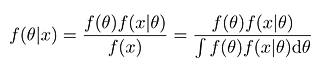 (This is for a continuous f; the discrete equivalent is much the same but sums over the set of outcomes rather than integrating.)
In general, what we are interested in is the posterior distribution, which is to say the estimate of the model parameter probabilities derived from the observed data. However, in order to get to that we always need to have a prior distribution, and this is one of the things that often draws criticism: the prior is an important part of the statistical model, but at some level it just has to be plucked out of nowhere. Priors are sometimes based on some external intuition about how the system works; other times they are just chosen for (relative) mathematical convenience.
However, this aspect is not quite as questionable as it may seem. While the prior will certainly distort the posterior when there is little data, as more observations are added the prior becomes less and less important. In the limit, the data dominates and the posterior should always ultimately converge towards the correct value. Since estimating a probability distribution from very small quantities of data is a dubious proposition anyway, the complaint reduces to one of potential methodological inefficiency -- a badly chosen prior may lead to very slow convergence -- rather than actual invalidity.
A problem with Bayesian methods is that they typically require the integration of complex functions for which no analytic method exists.3 Numerical approximations may be used instead, but these are computationally difficult and have only really become practical with rise of digital computers.
A common technique for sampling from such distributions without explicit integration is Monte Carlo simulation, usually in the form of Markov Chain Monte Carlo (MCMC). What this means is that we take a random walk through the state space, with each step being assessed according to the ratio of densities between the current position and the proposed next. The distribution of states hit by the walk converges to the target distribution itself, so the chain makes a reasonable approximation thereof (after some initial burn-in period).
Among other areas of relevance to bioscience, MCMC techniques have been applied to problems in population genetics and phylogeny. An example of the former is estimating the mutation rate in a population given observations of the alleles at one or more neutral loci. In this case, the Markov Chain is used to walk the space of possible coalescence trees (ie, how the mutations occur as you go back through the generations) and associated mutation rates, converging to a distribution for the latter (the actual trees are integrated out of the model).
Phylogenetic applications are related -- organising genes or species into taxonomic trees -- but are concerned with the tree topology, making for a rather more complicated model -- one that estimates more parameters and requires more priors. Consequently the results -- given, say, as a 95% credibility set of most likely trees, along with posterior clade probabilities identifying the branch groupings that occur in the largest number of tree candidates -- are potentially more suspect.
(This is for a continuous f; the discrete equivalent is much the same but sums over the set of outcomes rather than integrating.)
In general, what we are interested in is the posterior distribution, which is to say the estimate of the model parameter probabilities derived from the observed data. However, in order to get to that we always need to have a prior distribution, and this is one of the things that often draws criticism: the prior is an important part of the statistical model, but at some level it just has to be plucked out of nowhere. Priors are sometimes based on some external intuition about how the system works; other times they are just chosen for (relative) mathematical convenience.
However, this aspect is not quite as questionable as it may seem. While the prior will certainly distort the posterior when there is little data, as more observations are added the prior becomes less and less important. In the limit, the data dominates and the posterior should always ultimately converge towards the correct value. Since estimating a probability distribution from very small quantities of data is a dubious proposition anyway, the complaint reduces to one of potential methodological inefficiency -- a badly chosen prior may lead to very slow convergence -- rather than actual invalidity.
A problem with Bayesian methods is that they typically require the integration of complex functions for which no analytic method exists.3 Numerical approximations may be used instead, but these are computationally difficult and have only really become practical with rise of digital computers.
A common technique for sampling from such distributions without explicit integration is Monte Carlo simulation, usually in the form of Markov Chain Monte Carlo (MCMC). What this means is that we take a random walk through the state space, with each step being assessed according to the ratio of densities between the current position and the proposed next. The distribution of states hit by the walk converges to the target distribution itself, so the chain makes a reasonable approximation thereof (after some initial burn-in period).
Among other areas of relevance to bioscience, MCMC techniques have been applied to problems in population genetics and phylogeny. An example of the former is estimating the mutation rate in a population given observations of the alleles at one or more neutral loci. In this case, the Markov Chain is used to walk the space of possible coalescence trees (ie, how the mutations occur as you go back through the generations) and associated mutation rates, converging to a distribution for the latter (the actual trees are integrated out of the model).
Phylogenetic applications are related -- organising genes or species into taxonomic trees -- but are concerned with the tree topology, making for a rather more complicated model -- one that estimates more parameters and requires more priors. Consequently the results -- given, say, as a 95% credibility set of most likely trees, along with posterior clade probabilities identifying the branch groupings that occur in the largest number of tree candidates -- are potentially more suspect.
1 All a bit biblical, isn't it? Perhaps appropriate for the Reverend Bayes, not that he actually has much to do with the stuff for which modern statisticians take his name in vain.
2 Popular failure to appreciate this fairly basic statistical notion is a constant boon to tabloid journalists, especially those of the hang 'em and flog 'em persuasion. Consider, for example, the extremely low prevalence of being a serial killer, and the low accuracy of identifying same, and then imagine just how much of the country you'd have to lock away on spec in order to preempt even a single murder.
3 Although the models can sometimes be structured into a hierarchy of conditionally-related submodels that are individually more tractable.
Posted by matt at April 23, 2007 02:22 PM
Comments
Something to say? Click here.